Introduction
FITfileR is an R package to read FIT files produced by fitness tracking devices like Garmin Edge cycle computers or sports watches. The intention for FITfileR is to use native R code to read the files directly, with no reliance on the FIT SDK or other FIT parsing tools. As such it should be platform independent, and not require any additional software outside of a working version of R.
Installing and loading the library
Currently FITfileR is only available on Github, and can be installed using the remotes package.
if(!requireNamespace("remotes")) {
    install.packages("remotes")
}
remotes::install_github("grimbough/FITfileR")
Once the package is installed, you then need to load the library in your R session before it can be used.
Example fit files
FITfileR is distributed with several example FIT
files to test its functionality. These files can be found in the
extdata\Activities folder of the package, and you can see
the names of all the example files with:
list.files(system.file("extdata", "Activities", package = "FITfileR"))## [1] "garmin-edge530-ride.fit" "garmin-fenix6-swim.fit"
## [3] "garmin-fenix6-turbo.fit" "tomtom-runner3-ride.fit"
## [5] "zwift-turbo.fit"The names of these files indicate the manufacture and model name of the device it was recorded on, as well as the activity type. There are many other differences (e.g. connected sensors, recording frequency, software versions) that are not encapsulated in the file names.
Reading files
To demonstrate reading a FIT file we’re going to use the
garmin-fenix6-swim.fit file distributed with
FITfileR.
library(FITfileR)
fenix6_file <- system.file("extdata", "Activities", "garmin-fenix6-swim.fit",
                            package = "FITfileR")
We read files using the function readFitFile().
fenix6 <- readFitFile(fenix6_file)The resulting object is an object of type FitFile
containing all the data stored in the original FIT file. Typing the name
of the object will print some details about the file e.g. the time it
was created, the manufacturer and name of the device it was recorded on,
and the number of data ‘messages’ held within the file. Exactly what
is shown here will depend on the information available in the file, so
it may look slightly different for you.
fenix6## Fit File
## ├╴File created: 2020-08-28 10:03:37
## ├╴Device: garmin fenix6
## └╴Number of data messages: 2141Working with the data
If we want to do more than just print a summary of the FIT file to screen we need to use some accessor function to extract the data from our FitFile object. There are several ways to achieve this depending on the datatype you’re interested in.
Records - GPS, speed, altitude, etc
The data most often wanted from a fit file are the values such as
location, speed, altitude, etc recorded during an activity. Such data
are classed as records in the FIT specification and can be
retrieved from the FitFile object using using
records().
fenix6_records <- records(fenix6)
fenix6_records
## $record_1
## # A tibble: 6 × 10
## timestamp position_lat position_long distance enhanced_speed
## <dttm> <dbl> <dbl> <dbl> <dbl>
## 1 2020-08-28 10:03:37 46.8 9.85 0 0
## 2 2020-08-28 10:03:38 46.8 9.85 0 0
## 3 2020-08-28 10:03:39 46.8 9.85 0 0
## 4 2020-08-28 10:03:40 46.8 9.85 0 0
## 5 2020-08-28 10:03:41 46.8 9.85 0.01 0.009
## 6 2020-08-28 10:03:42 46.8 9.85 0.03 0.021
## # ℹ 5 more variables: heart_rate <int>, cadence <int>, temperature <int>,
## # cycles <int>, fractional_cadence <dbl>
##
## $record_2
## # A tibble: 651 × 10
## timestamp position_lat position_long distance enhanced_speed
## <dttm> <dbl> <dbl> <dbl> <dbl>
## 1 2020-08-28 10:03:43 46.8 9.85 0.1 0.069
## 2 2020-08-28 10:03:44 46.8 9.85 0.19 0.087
## 3 2020-08-28 10:03:45 46.8 9.85 0.3 0.111
## 4 2020-08-28 10:03:46 46.8 9.85 0.44 0.143
## 5 2020-08-28 10:03:47 46.8 9.85 0.6 0.164
## 6 2020-08-28 10:03:48 46.8 9.85 0.8 0.199
## 7 2020-08-28 10:03:49 46.8 9.85 1.02 0.217
## 8 2020-08-28 10:03:50 46.8 9.85 1.3 0.28
## 9 2020-08-28 10:03:51 46.8 9.85 1.6 0.301
## 10 2020-08-28 10:03:52 46.8 9.85 1.92 0.313
## # ℹ 641 more rows
## # ℹ 5 more variables: heart_rate <int>, cadence <int>, temperature <int>,
## # cycles <int>, fractional_cadence <dbl>
##
## $record_3
## # A tibble: 1 × 9
## timestamp position_lat position_long distance heart_rate cadence
## <dttm> <dbl> <dbl> <dbl> <int> <int>
## 1 2020-08-28 10:12:02 180. 180. 408. 140 36
## # ℹ 3 more variables: temperature <int>, cycles <int>, fractional_cadence <dbl>In this example we actually get a list with three
tibbles. This is because in this particular file there are
three distinct definitions of what a record contains. This
normally happens if data recording begins before a sensor (e.g. a heart
rate monitor) has been attached to a device, or GPS position has been
acquired, although sometimes the reason can be more opaque. In this
example it seems clear that we can use the second entry, which contains
the vast majority of the data. Note: sometimes the bulk of your data
may be spread across multiple tibbles in the list rather
than a single entry. See the “Plotting a route” section below for an
example of how to handle this.
Extracting common data types
In addition to the records() function,
FITfileR provides an number of other methods for
accessing commonly found message types. Currently, these include:
Accessing any data type
The FIT specification allows for 91 distinct message types, and
FITfileR does not include specific accessor functions
for each of these. To view a complete list of the message types stored
within a file you can use the function
listMessageTypes().
listMessageTypes(fenix6)## [1] "file_id" "device_settings" "user_profile" "zones_target"
## [5] "sport" "session" "lap" "record"
## [9] "event" "device_info" "activity" "file_creator"
## [13] "gps_metadata"We can see there are 13 different message types in the file above. If
a specific accessor method doesn’t exist for the message type you’re
interested in, you can use the function getMessagesByType()
and provide the message type name to the message_type
argument. The code below will extract all “zones_target” messages from
our file.
getMessagesByType(fenix6, message_type = "zones_target")## # A tibble: 1 × 5
## functional_threshold_power max_heart_rate threshold_heart_rate hr_calc_type
## <int> <int> <int> <chr>
## 1 275 184 0 percent_max_hr
## # ℹ 1 more variable: pwr_calc_type <chr>In this case zones_target is a single message that reports power and heart rate thresholds that were set on the device. One could imagine using these in conjunction with the records to measure how well the athlete performed relative to the pre-set threshold for this particular activity.
Example use cases
Plotting a route
edge530_file <- system.file("extdata", "Activities", "garmin-edge530-ride.fit",
                            package = "FITfileR")
edge530 <- readFitFile(edge530_file)
To plot locations we extract the longitude and latitude from our FIT
records. These data are found in record messages, and we use
records() to extract them. As before, we are returned a
list of tibbles. However, unlike the previous example there is no entry
that clearly holds almost all the data; there are two different
definitions for record messages with over one thousand data
points.
edge530_records <- records(edge530)

## report the number of rows for each set of record messages
vapply(edge530_records, FUN = nrow, FUN.VALUE = integer(1))
## record_1 record_2 record_3 record_4 record_5 record_6 record_7
## 3 197 7 9 7063 1326 22We probably don’t want to discard either of these, as even the
smaller one represents over 20 minutes of data recording. We can use
dplyr to try and merge all the messages together into a
single tibble regardless of their definition. Any entries
that are missing in certain messages will be filled with
NA. Note: this approach of binding rows does not always
work, as sometimes the data types within a column may change between
messages, but it is more often successful.
library(dplyr)

edge530_allrecords <- records(edge530) %>%
  bind_rows() %>%
  arrange(timestamp)

edge530_allrecords
## # A tibble: 8,627 × 23
## timestamp position_lat position_long distance altitude speed power
## <dttm> <dbl> <dbl> <dbl> <dbl> <dbl> <int>
## 1 2020-07-15 12:31:43 42.9 -0.00165 0 731. 1.26 65535
## 2 2020-07-15 12:31:44 42.9 -0.00164 1.35 731. 1.35 142
## 3 2020-07-15 12:31:45 42.9 -0.00162 2.82 731. 1.46 142
## 4 2020-07-15 12:31:46 42.9 -0.00160 4.55 731. 1.73 142
## 5 2020-07-15 12:31:47 42.9 -0.00158 6.65 731. 2.10 170
## 6 2020-07-15 12:31:48 42.9 -0.00154 9.81 731. 3.17 256
## 7 2020-07-15 12:31:49 42.9 -0.00149 14.0 731. 4.16 242
## 8 2020-07-15 12:31:50 42.9 -0.00144 18.3 731. 4.32 0
## 9 2020-07-15 12:31:51 42.9 -0.00139 22.3 731. 4.02 0
## 10 2020-07-15 12:31:52 42.9 -0.00135 25.8 731. 3.49 0
## # ℹ 8,617 more rows
## # ℹ 16 more variables: heart_rate <int>, temperature <int>,
## # accumulated_power <dbl>, left_right_balance <int>,
## # left_torque_effectiveness <dbl>, right_torque_effectiveness <dbl>,
## # left_pedal_smoothness <dbl>, right_pedal_smoothness <dbl>, cadence <int>,
## # fractional_cadence <dbl>, left_pco <int>, right_pco <int>,
## # left_power_phase <list>, left_power_phase_peak <list>, …We can then use dplyr::select() to extract the latitude
and longitude columns from our tibble, so we can pass them
easily to a plotting function.
We can now use the leaflet package to create an interactive map, with our route overlayed on top.
Comparing heart rate measurments between devices
The package comes with two example fit files, recorded during a Zwift activity in 2021. They are of the same ride and record the same rider, but some of the data recording was carried out on two different devices so they could be compared. Specifically, a Garmin heart rate strap and and Elite Direto trainer were linked to Zwift for recording heart rate and power, alongside a Garmin Fenix 6 wrist based heart rate monitor and Assioma Duo pedals measuring the same properties.
Here we compare the heart rates recorded with two devices, to see how consistent they are with each other.
First we need to locate the two files and read them into R:
garmin_file <- system.file("extdata", "Activities", "garmin-fenix6-turbo.fit",
                            package = "FITfileR")
zwift_file <- system.file("extdata", "Activities", "zwift-turbo.fit",
                            package = "FITfileR")

garmin <- readFitFile(garmin_file)
zwift <- readFitFile(zwift_file)
We then use records() to extract the appropriate
messages from the two files. Since there’s a lot of data in addition to
the heart rate readings we’re interested in, we use functions from
dplyr and tidyr to combine the heart
rate data into a single data frame, and make it into a ‘long’ format
suitable for plotting with ggplot2.
garmin_records <- records(garmin) %>%
    bind_rows() %>%
    arrange(timestamp)
zwift_records <- records(zwift)

hr_table <- inner_join(garmin_records, zwift_records, by = "timestamp") %>%
  select(timestamp, Garmin = heart_rate.x, Zwift=heart_rate.y) %>%
  tidyr::pivot_longer(cols = Garmin:Zwift, names_to = "device", values_to = "heart_rate")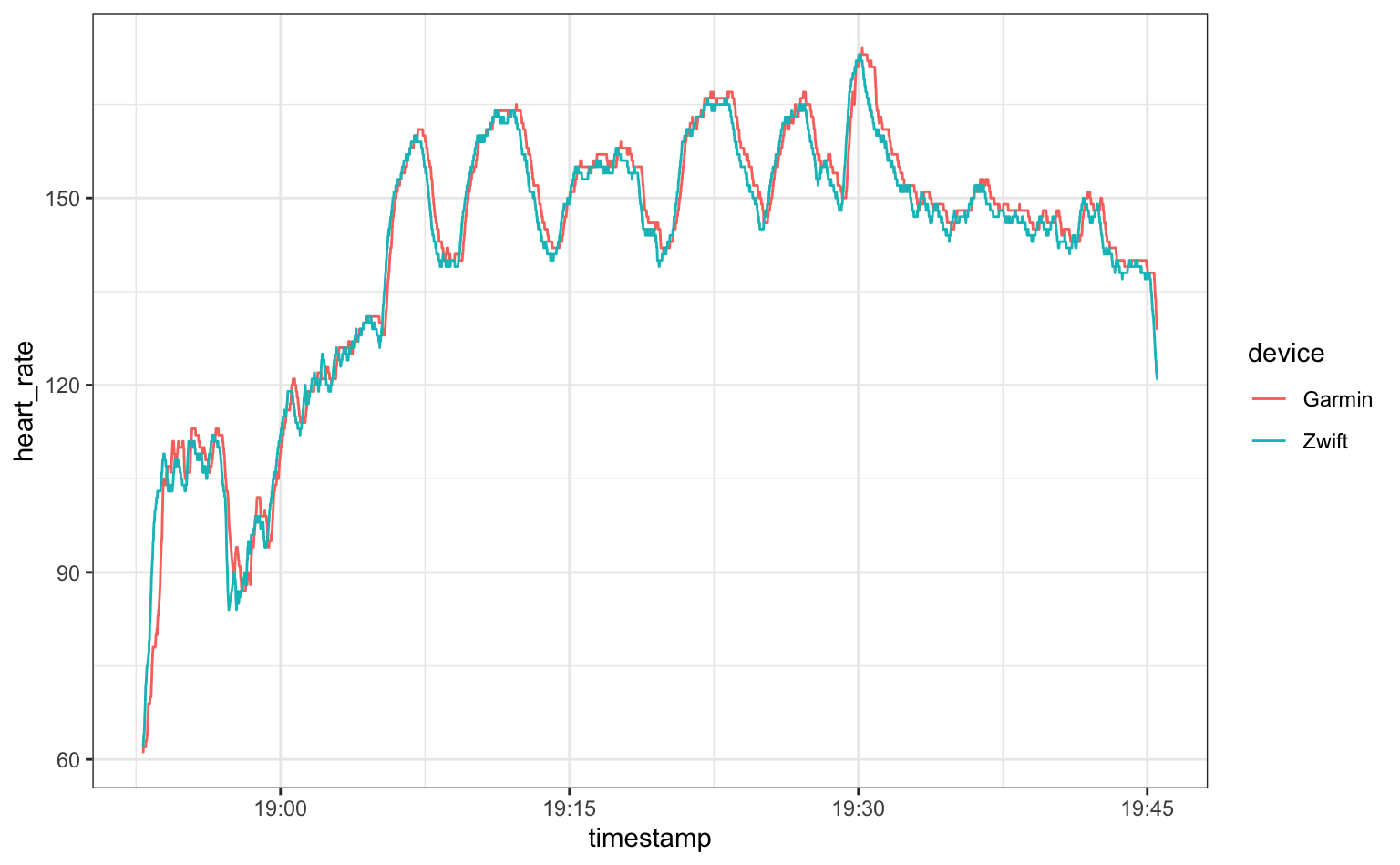
The two heart rate monitors correspond well over the duration of the workout. There seems to be a 1-2 second lag in the wrist-based monitor (Garmin), but the high and low values track really well. Based on this I’d have no issue relying on the Fenix 6 heart-rate monitor for my training.
We can also consider the difference between the two measurements both at each common time point and also as a rolling mean over a 60 second window.
library(zoo)

hr_differences <- hr_table %>%
  pivot_wider(id_cols = timestamp, names_from = device, values_from = heart_rate) %>%
  mutate(hr_diff = Garmin - Zwift,
         Garmin_hr_zone = cut(Garmin, breaks = seq(0,200,20))) %>%
  mutate(hr_60 = zoo::rollmean(hr_diff, k = 60, fill = NA))

ggplot(hr_differences, aes(x = timestamp, y = hr_diff)) +
  geom_point(aes(col = Garmin_hr_zone)) +
  geom_line(aes(y = hr_60), col = "grey40", lwd = 1.6, alpha = 0.7) +
  geom_abline(intercept = 0, slope = 0) +
  theme_bw() +
  ylab("Heart Rate Difference\n+ve Chest Strap Greater / -ve Wrist Watch Greater") +
  scale_colour_brewer(palette = "PRGn")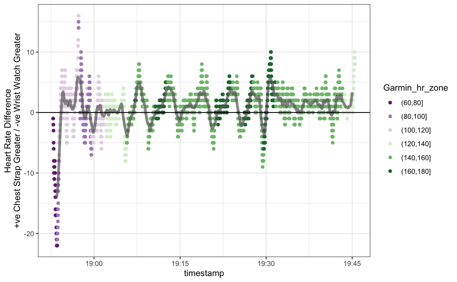
For the most part the readings are quite similar between the two devices. Just looking at the plot, it seems there are more points above the zero line, indicating that the chest strap records slightly higher values on average, but the difference is generally within 5 beats-per-minute. Based on the colouring it looks like the largest differences occur when the heart-rate is high.
More details
In this section we describe a few more of the implementation details of FITfileR and some of the choices made in presenting the data in an R session.
Data types and units
Much of the data contained in FIT files is not stored in the formats
that you might instinctively expect or that see on the display of the
device the file was recorded on. For example, the elapsed time of an
activity isn’t stored in seconds, but rather milliseconds, and this
value needs to be scaled to get the time in seconds. Other data types
require more complex processing. The latitude and longitude positional
information, which is not stored as decimal degrees
(e.g. 42.87342) but rather as a signed 32-bit integer
(e.g. 511512370) representing “semicircles”, needs to be
converted by multiplying by the scaling factor
.
Similarly, text information such as the activity type or device
manufacturer isn’t stored directly as the string “run” or “Garmin” but
as an integer that maps to an entry in a table of sports or
manufacturers respectively.
More details of the data types can be found in the
Profile.xlsx file that is provided as part of the FIT SDK.
FITfileR has its own internal representation of this
file, and will try to convert many data types automatically. In most
cases it is possible to find the units for the values
FITfileR is displaying via the units
attribute. This will either be printed to screen alongside the contents
of a data column, or you can extract the units attribute
directly.
garmin_session <- getMessagesByType(garmin, "session")
## show the latitude of the start position
garmin_session$start_position_lat
## [1] 180
## attr(,"units")
## [1] "degrees"
## extract the units for the total ascent value
attr(garmin_session$total_ascent, "units")
## [1] "m"This automatic conversion works for many of the more common fields
based around timestamps, GPS positions, distances, speeds, and probably
many more. However the FIT specification is large and it is likely there
are common data types that I have not encountered in one of my own FIT
files. If you come across a field that is entirely NA then
it is likely that your file includes a data type that
FITfileR does not currently support. Please open an
issue at GitHub and I
will try to add the required functionality.
Session Info
## R version 4.4.2 (2024-10-31)
## Platform: aarch64-apple-darwin20
## Running under: macOS Sonoma 14.7.2
##
## Matrix products: default
## BLAS:   /Library/Frameworks/R.framework/Versions/4.4-arm64/Resources/lib/libRblas.0.dylib
## LAPACK: /Library/Frameworks/R.framework/Versions/4.4-arm64/Resources/lib/libRlapack.dylib;  LAPACK version 3.12.0
##
## locale:
## [1] en_US.UTF-8/en_US.UTF-8/en_US.UTF-8/C/en_US.UTF-8/en_US.UTF-8
##
## time zone: UTC
## tzcode source: internal
##
## attached base packages:
## [1] stats     graphics  grDevices utils     datasets  methods   base
##
## other attached packages:
## [1] ggforce_0.4.2   zoo_1.8-12      ggplot2_3.5.1   tidyr_1.3.1
## [5] leaflet_2.2.2   dplyr_1.1.4     FITfileR_0.1.11
##
## loaded via a namespace (and not attached):
##  [1] sass_0.4.9         utf8_1.2.4         generics_0.1.3     lattice_0.22-6
##  [5] digest_0.6.37      magrittr_2.0.3     evaluate_1.0.3     grid_4.4.2
##  [9] RColorBrewer_1.1-3 fastmap_1.2.0      jsonlite_1.8.9     purrr_1.0.2
## [13] crosstalk_1.2.1    scales_1.3.0       tweenr_2.0.3       codetools_0.2-20
## [17] jquerylib_0.1.4    cli_3.6.3          rlang_1.1.5        polyclip_1.10-7
## [21] bit64_4.6.0-1      munsell_0.5.1      withr_3.0.2        cachem_1.1.0
## [25] yaml_2.3.10        tools_4.4.2        colorspace_2.1-1   vctrs_0.6.5
## [29] R6_2.5.1           lifecycle_1.0.4    fs_1.6.5           htmlwidgets_1.6.4
## [33] bit_4.5.0.1        MASS_7.3-61        pkgconfig_2.0.3    desc_1.4.3
## [37] pkgdown_2.1.1      pillar_1.10.1      bslib_0.8.0        gtable_0.3.6
## [41] Rcpp_1.0.14        glue_1.8.0         xfun_0.50          tibble_3.2.1
## [45] tidyselect_1.2.1   knitr_1.49         farver_2.1.2       htmltools_0.5.8.1
## [49] rmarkdown_2.29     labeling_0.4.3     compiler_4.4.2